Quest for a gremlin-free Sales Analysis-Cube
by P Barber (January
2010)
This short paper provides an outline of the author’s quest to create a gremlin-free sales-data analysis cube. Early investigation revealed computation problems associated with particular data conditions, but the real challenge was understand why the numbers calculated at different levels did not add-up.
The authors quest for a gremlin-free Sales Analysis-Cube began in 1995 when he moved to a central role in GE Lighting (Europe) Ltd. This division of General Electric Ltd, (USA, not to be confused with the UK Company with a similar name) had brought together the large East European light-source sales and manufacturing facilities of Tungsram, based in Hungary, with the Western European light-source markets of Thorn Lighting and Sivi of Italy. The result of this combination was a lighting conglomerate which sold in excess of 23,000 product lines (64,000 if components and obsolete products were included), to 4,000 customers, delivering to 32,000 branches, in 10 market segments, 9 sub-sales regions, across 13 countries, and Invoicing in16 different currencies. This complexity led to a demand to be able to attribute sales and margin variances in a number of different ways:
a) By Country Affiliate
b) By Product Line, by Product Group, by SKU
c) By Marketing Channel, by Customer Group, by Customer, by Branch
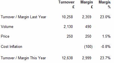
Jack Welch, then CEO of General Electric, favoured the use of what he termed the Margin Waterfall Report for monitoring the financial performance of divisions.
The top row of this report indicated the Sales and Margin for the previous period. Subsequent rows then tracked the factors which led to the changes in sales and margin from one period to another using three columns:
a) Sales in currency
b) Margin in currency, and
c) Margin as a percentage of Sales.
The second row of the report indicated the amount of change attributable to volume, and assumed that the percentage margin was the same as in the previous period.
In the simplified example, shown below, the third line shows the effect of changes in sales price. It can be seen that changes in price affect the margin directly (as shown by the fact that the values shown in the turnover and margin columns are equal)
In practice the number of lines in the report was expanded to show the factors that were relevant, but the report would typically include material cost inflation, materials productivity, labour productivity, exchange rate, etc. The total at the bottom of the Margin Waterfall Report was equal to the Sales and Gross margin for the current period.
A simplified illustration is shown below:
The author’s task at GE Lighting ( Europe) was to provide the monthly variances for volume, price and exchange, and to explain where and how they had arisen. Previously there had been a $13 million hole in the analytics.
Initial analysis indicated that the quality of data was poor so a six-sigma project was launched to address this issue. It was found that the conventional price variance calculations were unstable. As with chemical instability, on occasions the results of the variance calculations were found to be catastrophic, producing variances far in excess of their real importance, resulting in the wasting of significant senior-management time.
On one occasion a batch of Compact Fluorescent Lamps had been shipped to a distributor in < st1:country-region > < st1:place > Belgium < /st1:place > . A few of these lamps were later returned, but the accounting system left behind a small positive value in Belgian Francs (+0.04 BEF). Because of fluctuations in the dollar exchange rate, this small amount was converted into a difference of minus $6.58. In those days the system used the local currency and dollar amounts to determine an average exchange. The system duly calculated an exchange rate of minus $164.5/BEF (-$6.58 / 0.04 = -164.5 ) and as a consequence this small 0.04 BEF difference was reported as a very large $3,300,000 price variance.
Analysis of this transaction identified that the method of calculating the exchange rate was poor: it was not possible to have a negative exchange rate. The process was therefore changed and in future a look-up table was used for determining the exchange rate.
Another significant source of error was caused by unmatched credit notes. These occurred when a credit note applicable to a previous year was entered into the current year. The effect was to achieve a condition where the quantity sold is positive and the net sales are negative, or vice versa. Either way this condition results in the calculation of a negative sales-price – which like the negative exchange rate is a difficult concept to comprehend – but not withstanding, the arithmetic becomes unstable. The solution here was to monitor for this condition by initial screening of the data, and to ensure that all occurrences were isolated. Logically the full variance associated with these items, net of exchange variance, falls into price variance.
Value-only credit notes produced a divide-by-zero-error when the sales-price-each is calculated. So the process was modified so that value-only credit notes were identified and allocated to price variance at the beginning of the process.
Developing a process
An important element of the Six-Sigma approach is to fix the process. This was achieved by controlling the process using an Access Database. Although Access was not considered the ideal tool for the full implementation, because of size limitations, it did however provide a means of Fast-Prototyping a system, which could then be implemented in an Oracle system. Because the basic calculations had previously been attempted using Excel spreadsheets, a significant processing speed advantage was achieved when these processes were converted to run in Access. The added advantage was that data could be down-loaded from the main SAP accounting system, enabling greater visibility of sales transactions. The elimination of errors, which were inherent in the spreadsheets, was also a factor in improving the speed and reliability of the process. This time could then be spent in identifying other sources of error, and modifying the process to remove their impact.
The Six-Sigma approach stresses the importance of getting things right first time. Invariably it is the few errors that absorb management time, and not the millions of transactions which are ok. If you get into your car and start the engine and every thing is working ok, you get to your destination on time and you never give your car a second though. However, if you get in your car, turn the ignition and hear a muffled click, followed by a humph… sort of noise, and then silence, then you have got a problem. You have got a car to fix, an appointment to keep, you are going to be late, and you are going to experience a whole lot of problems that were not previously on your agenda. Getting the process right first time really helps.
Problems with
drilling into the data
Perhaps the greatest challenge was understand why numbers calculated at different levels did not add-up. If we calculated the Price and Volume variances at the total company level we got one answer. If we then tried to analyse the data at the next level down and then add up the results we got a different answer. It was just not possible to cut-and-dice the data to determine where all the variances were coming from.
Recognition of this problem was not new, Anthony (1970) stated that “If revenue is analysed by individual products, or by individual geographic regions, a mix variance inevitably arises. Failure to appreciate this fact can lead to great frustration in trying to make the figures add-up properly.”
Anthony (1970) saw variance analysis as a top-down process, where the Analyst identifies a significant variance at the top-level, and then drills-down into the data to determine the reason for the variance. Anthony implies that the deeper the analyst drills the data the greater the amount of “mix” becomes.
Tops down Analysis
I must admit that the case for Tops-down analysis is deeply ingrained into my psyche. I have spent the best part of 30 years drilling into data to determine the root cause of a variance that appeared at the top level. This is the way the Financial Analyst works, isn’t it? So there is an in-built view that the answer calculated at the Total Company level is correct, and that the effect of “Mix” becomes apparent as you drill down and “Cut-and-Dice” the data, as Anthony (1970) said, “This was to be expected”. My boss expressed the view that “mix did not exist at the single SKU by Customer level, but it did exist at the aggregated level”, but he was quickly silenced. The concept that you got a different answer every time you cut the data was impossible – imagine trying to tell that to the boss! - We therefore opted for the “Top-down” approach. (Modification of this view took a further six or so years)
Mix v Level
Adjustment
The traditional materials Mix calculation shown in Text Books, such as Anthony (1970); Bhimani etal. (2008); Hasen & Mowen (2006); etc., did not seem to be helpful in analysing the differences between the levels of analysis, in that a volume movement on one SKU would result in a mix-variance being applied to every SKU in the data set, and not just the single SKU that had changed.
After a lot of mathematical manipulation an equation was developed which seemed to give the result we were looking for. (viewed as the Analysts equivalent to E = MC2 and clearly worthy of a Nobel Prize). It was later found that this equation had been proposed by Hasseldine (1967).
The effect of the Level-Adjustment calculation was to transfer variance between the Price-variance and Volume-variance columns: the equation was of the form:
(QiT – QiL)(PiL – Pave) = Level Adjustment
Where:
QiT = elemental quantity sold this year
QiL = elemental quantity sold last year
PiL = elemental price-each last year
Pave = the average price-each for the whole set
The formula above effectively shows the difference between Volume-variance calculated at the elemental level [(QiT – QiL)PiL] and a Volume-variance calculated at the aggregate level [(QiT – QiL)Pave].
At the time I left GE Lighting (Europe) in October 2001 the Six-Sigma team were planning the launch of a project to determine who was responsible for this “Level Adjustment or Mix variance”. Shortly after that the head-office was relocated to Budapest , and I never did find out if they ever identified the culprit!
Review of the
Literature
Having, as they put it; “gone on to pursue other interests”, I then began to turn my attention to a number of questions that had been raised during the quest for the “Gremlin-Free Analysis Cube”.
A number of references (supplied by Professor Colin Drury of Huddersfield University ), which, although perhaps a bit old, dealt with problem of “Mix” and the fact that the numbers did not add up:
a) Peles (1986) stated that : These latter variances (mix) have a defect which can led to dysfunctional decisions. Since these variances are based on an average unit price which varies with respect to the unit of measurement selected, the same real events can appear as positive or negative variances.
b) Bastable and Bao (1988) stated that: due to imperfect measurement sales-mix variances have the potential for doing more harm than good. And that the wise course would seem to be to refrain from such quantification.
c) Chumachenko (1968) compared the sales-mix variance calculations of US and Soviet methods and illustrates seven different methods. He states that: when a company produces several different products measuring the volume of sales in physical units becomes devoid. He seems to favour the Soviet approach, which is to use Sales (£,$,etc) as a means of monitoring volume.
d) Malcom (1978) concluded that aggregated products should have margins as homogeneous as possible and that great care must be exercised in reports to indicate the level to which any mix variance applies.
e) Gibson (1990) states that: A telling condemnation of the traditional mix variance computation is its necessary reliance on an arbitrarily defined unit of product. The numerical expression of the total quantity of products is dependent on the unit of measure chosen (what is the total of one kilogram of grapes plus one handful of bananas?) Applications of traditional procedures will result in different apportionment to quantity and mix variances when different units of measure are used.
f) Zannetos (1963) considered that there is a tendency to confuse mathematical correctness with accounting validity and utility. He states that: Accounting is not an exact science but a utilitarian tool full of rules of reason. Mathematics on the other hand is a universal tool based on logic that is not influenced by the immediate operational environment. Consequently we must not automatically conclude that we can transfer validity and managerial import through mathematical sanction alone.
While I would agree with Zannetos that the solution to an analysis problem cannot be separated from the data and that the blind application of a formula is to be discouraged, I am not sure that I would be prepared to dispense with the mathematics. What is clear from the literature, above, is that there has been dissatisfaction with the concept of sales-mix-variance for some time and that much of this dissatisfaction centres on the choice of units. Some, like Chumachenko (1968), favour a sales (currency) measure rather than units sold. However, it is Gibson (1990) who identifies the real problem. As he puts it: “what is the total of a kilogram of grapes and a hand of bananas?”
Level Adjustment is
Computational Error
The GE Lighting analysis cube combined the sales of small automotive lighting components, at a sales price of $0.07 each, along with CID2500 Studio lamps that had a selling price of $330 each. This difference in selling prices led to very significant errors in calculating the Price-Volume variances, at the various levels of aggregation demanded by the business. In hindsight, it would have been correct to calculate these variances at the lowest possible level and to then add the low-level price and volume variances, to provide the best estimate of the aggregated variance. At least, then the numbers would add up.
And it can be seen that my boss, who expressed the view that mix did not exist at the elemental level, only at the aggregate level, was in fact correct. Sales-Mix does not exist and the difference you find when drilling down into the data is in fact Computational Error. The challenge is to create data sets which are homogeneous. The (most) correct result is obtained by summing the low level Price and Volume variance to determine the total variance for the consolidated level. Once again, the devil is in the detail.
References
Anthony, Robert N. 1970. Management Accounting: Text and Cases, Richard D. Irwin, Inc.
Barber P. L. (2009) Re-examination of sales price and volume variance, solutionuk.com
Bastable C.W. and Bao, D.H. (1988), The fiction of sales mix and sales quantity variances, Accounting Horizons, June, 10-17.
Bhimani A., Horngren C.T. Dator S.M., Foster G. (2008) Management and Cost Accounting, Prentice Hall p587-589
Gibson B. (1990), Determining meaningful sales relational (mix) variances, Accounting and Business Research, Winter, 35-40.
Hansen D.R., Mowen M.H. (2006), Cost Management Accounting and Control, Thomson South-Western p407-409, 746
Hasseldine C. R. (1967), Mix and yield variances, The Accounting Review, 42(3), July, p497-515
Malcome R. E. (1978), The effect of product aggregation in determining sales variances, The Accounting Review, January, p162-169
Peles Y. C. (1986), A note on yield variance and mix variance, The Accounting Review, Vol LX1, No.2, April 1986 p325-329
Zannetos Z S (1963), On the Mathematics of Variance Analysis, The Accounting Review, July, 528-533