Fitting the
Humphreys Distribution to a Dataset
by P Barber ( January 2010)
INTRODUCTION
1. A significant challenge with simulation modelling is to be able to
determine the distribution of any resultant data set.
2. Packages such as Crystal Ball (http://www.oracle.com/appserver/business-intelligence/crystalball/index.html)
or EasyFit (www.matwave.com) provide a
means of determining the best-fit, from many of the common distributions
available, but unfortunately the Humphreys distribution (see section 32) is not included within the
libraries of these packages.
3. This paper sets out an iterative process for
determining the NMX parameters and then goes on to outline a method of
estimating these parameters directly from measurements of the dataset Mean,
Standard Deviation, Skew and Kurtosis. ( see section 16)
ITERATIVE
METHOD OF FITTING A DISTRIBUTION
4. The Iterative Method utilises the Anderson
Darling test (see section 51)
.
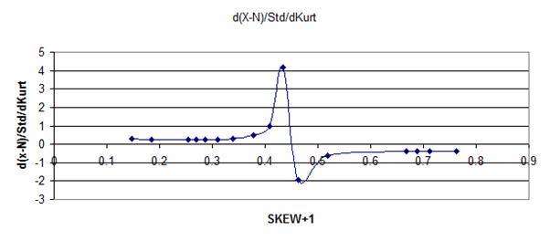
5. At the beginning of the iterative process an
estimate of the NMX parameters of the data-set is made. In this example
parameters of N=126.479, M=170.162,
X=198.597 have been assumed, and this results in an Anderson Darling statistic
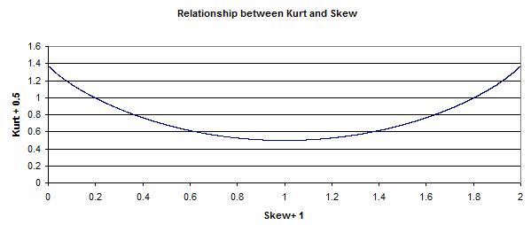
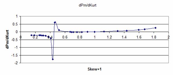
of AD = 108.08
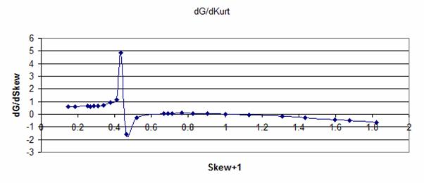
|
N
= |
126.479 |
|
M
= |
170.162 |
|
X
= |
198.597 |
|
AD
= |
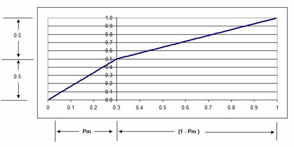
108.082605 |
6. The
value of the first parameter (N) is then increased by (0.001). The results of
the first and second trial are shown below.
|
N
= |
126.479 |
126.48 |
|
M
= |
170.162 |
170.162 |
|
X
= |
198.597 |
198.597 |
|
AD
= |
108.082605 |
108.113858 |
|
Mvt
AD= |
|
0.031253 |
7. From
the above it can be seen that the effect has been to increase the value of AD
by 0.031253, since it is desired to decrease the value of AD it is deduced that
the value of the first parameter (N) should have been reduced, rather than
increased.
|
N
= |
126.479 |
126.478 |
|
M
= |
170.162 |
170.162 |
|
X
= |
198.597 |
198.597 |
|
AD
= |
108.082605 |
108.051358 |
|
Mvt
AD= |
|
-0.031247 |
8. The
process of reducing the value of (N) is then repeated until three iterations,
providing four data elements, has been completed.
|
126.479 |
126.478 |
126.477 |
126.476 |
|
170.162 |
170.162 |
170.162 |
170.162 |
|
198.597 |
198.597 |
198.597 |
198.597 |
|
108.082605 |
108.051358 |
108.0201174 |
107.988883 |
|
|
-0.031247 |
-0.031241 |
-0.031235 |
9. The
next stage is to plot the values of AD against the moving parameter (N),
fitting a ‘Polynomial Order 2’ trendline and using the fitted equation to
calculate the turning point.
The data we have is:
|
N
= |
126.479 |
126.478 |
126.477 |
126.476 |
|
AD
= |
108.082605 |
108.051358 |
108.020117 |
107.988883 |
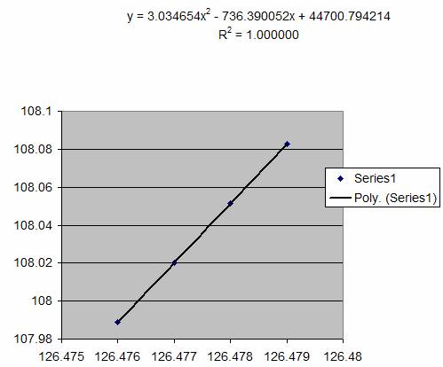
10. The
equation of the trendline is of the form:
Y = aX2 + bX + c
And the turning point occurs when dY/dX = 0
Differentiating the equation above we have:
dY/dX = 2aX +b = 0
Hence the turning point occurs when:
X = -b / 2a
The values found in the fitted trendline were:
a = 3.034654
b = - 736.390052
and if we substitute these into the equation:
X = -b / 2a
We get X = 736.390052/(2 x 3.34654) = 121.330
11.
Setting N = 121.330 we get a results which reduces the AD statistic from
107.988 to 17.5667
|
N
= |
126.479 |
126.478 |
126.477 |
126.476 |
121.33 |
|
M
= |
170.162 |
170.162 |
170.162 |
170.162 |
170.162 |
|
X
= |
198.597 |
198.597 |
198.597 |
198.597 |
198.597 |
|
AD
= |
108.082605 |
108.051358 |
108.0201174 |
107.988883 |
17.56672132 |
|
Mvt
AD= |
|
-0.031247 |
-0.031241 |
-0.031235 |
-90.422161 |
12.
Holding the parameters N and X constant the process is then repeated
with M.
|
N
= |
121.33 |
121.33 |
121.33 |
121.33 |
|
M
= |
170.162 |
170.161 |
170.16 |
170.159 |
|
X
= |
198.597 |
198.597 |
198.597 |
198.597 |
|
AD
= |
17.566721 |
17.546337 |
17.52596903 |
17.505617 |
|
Mvt
AD= |
|
-0.020384 |
-0.020368 |
-0.020352 |
13. With
the four data elements being
|
M
= |
170.162 |
170.161 |
170.16 |
170.159 |
|
AD
= |
17.566721 |
17.546337 |
17.525969 |
17.505617 |
Which when plotted:
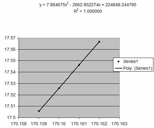
and if we substitute the equation parameters
into the turning point equation:
X = -b / 2a
We get X = 2662.952274/(2 x 7.884675) = 168.869
Insertion of this value results in a reduction
in AD from 17.505617 to 4.4608879
|
N
= |
121.33 |
121.33 |
121.33 |
121.33 |
121.33 |
|
M
= |
170.162 |
170.161 |
170.16 |
170.159 |
168.869 |
|
X
= |
198.597 |
198.597 |
198.597 |
198.597 |
198.597 |
|
AD
= |
17.566721 |
17.546337 |
17.52596903 |
17.505617 |
4.460887915 |
|
Mvt
AD= |
|
-0.020384 |
-0.020368 |
-0.020352 |
-13.044729 |
14. The
process is then repeated holding parameters N and M constant while adjusting X.
Once four iterations have been completed the data is used to construct a
trendline, calculate the turning point and reduce the value of AD further.
Repeating the process until no further reduction can be achieved.
|
X
= |
198.597 |
198.596 |
198.595 |
198.594 |
|
AD
= |
4.460887915 |
4.459631 |
4.458380154 |
4.457134 |
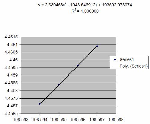
and if we substitute the equation parameters
into the turning point equation:
X = -b / 2a
We get X = 1043.546912/(2 x 2.630468) = 198.358
Which when substituted yields a further
reduction in the value of AD.
|
N
= |
121.33 |
121.33 |
121.33 |
121.33 |
121.33 |
|
M
= |
168.869 |
168.869 |
168.869 |
168.869 |
168.869 |
|
X
= |
198.597 |
198.596 |
198.595 |
198.594 |
198.358 |
|
AD
= |
4.460887915 |
4.459631 |
4.458380154 |
4.457134 |
4.311477132 |
|
Mvt
AD= |
|
-0.001257 |
-0.001251 |
-0.001246 |
-0.145657 |
15.
While it can be seen that the above method provides a method of fitting
the NMX parameters of the Humphreys Distribution to a data-set, the method
involves a significant number of iterations to achieve a final convergence,
particularly since the rate of convergence declines with each iteration, as can
be seen above. An alternative method, utilising the measurable parameters of
the data-set: Mean, Standard Deviation, Skew and Kurtosis.
ALTERNATIVE MEANS OF FITTING A DISTRIBUTION
16. The
parameters Mean, Standard Deviation, Skew and Kurtosis of a data-set can be
measured using standard Excel Functions. It should be noted however that the
values of Skew and Kurtosis vary
slightly with variations in the size of the data sample. Skew is a measure of
the third standardised moment of the data-set while Kurtosis is a measure of
the fourth standardised moment. As the size of the data-set is increased more
values are included ‘in the tails’ of the distribution, and these affect the
calculation of these two variables. To overcome this problem a standard
data-set with N= 10,000 elements was employed.
17.
Investigation of fitted data sets reveals that a number of relationships
exist, namely:
a) Pm and Skew
b) (Mean – M)/standard deviation and Skew
c) (X – N)/standard deviation and Kurtosis
d) (X – N)/standard deviation and Skew
Pm
and Skew
18. The relationship between Pm and Skew was
found to be:
(Mean
– M)/standard deviation and Skew
19. The relationship between (Mean –
M)/standard deviation and Skew is shown below.
(X –
N)/standard deviation and Kurtosis
20. The relationship between (X –
N)/standard deviation and Kurtosis is shown below.
(X – N)/standard deviation and Skew
21. The relationship between (X –
N) / standard deviation and Kurtosis is shown below.
22.
Using the above equations it was possible to develop a set of lookup tables
which would predict the NMX parameters for data-sets which possessed a
Humphreys Distribution. Three lookup tables were established based upon Skew+1
(SKEW+1 to unsure that all the values in the table were positive) and these
provided the following factors:
a)
Pm
b) G
= (Ave – M) / Std
c) H
= (X – N) / Std
Where:
Ave
= the Average or Mean of the data-set
Std
= the Standard Deviation of the data-set
Estimates
of the NMX Humphreys Distribution could then be estimated from the above
equations as follows:
a) M
= Ave – (G x Std)
b) N
= M – (Pm x H x Std)
c) X
= (H x Std) + N
23.
Although the above relationships provide a means of predicting the NMX
parameters for data-sets that possess a Humphreys Distribution, the above
relationships were not sufficient to provide the best-fit, when the underlying
distribution was different. A number of tests were carried out using data
created with a Beta Distribution and the following additional relationships
involving changes in Kurt were established.
24. Firstly for data which can be fitted closely
to a Humphreys Distribution, it was found that there was a relationship between
Skew and Kurt, as shown below.
25. However, it was found that the relationship
between Skew and Kurt changed when the data-set differed from the Humphreys
Distribution. The plots below show how differences in the value of Kurt (dKurt)
could be related to changes in the lookup table factors:
Pm,
G=
(Ave – M) / Std and
H =
(X – N) / Std
26. These relationships were used to create a
lookup table which would predict the NMX parameters over a wider range of
data-sets. However, it should be noted that in creating the lookup tables it
was assumed that the relationships between data points was linear. With the
limited number of data points employed in the trial it is therefore inevitable
that some inaccuracy will occur. However, it is considered that the method
provides a useful means of predicting the NMX parameters, which can then be
checked using the Anderson Darling statistic and if necessary further iteration
will yield a result close to the best fit.
APPLICATION OF LOOKUP TABLES
27. The section below illustrates the process for estimating NMX parameters using the developed Lookup Tables. (down-load table)
The
parameters for a data set have been measured as follows:
Mean
(Ave) = 123.0769
Standard
Deviation = 15.38512
Skew = 0.823478
Kutosis = 0.278257
Then
(Skew+1) = 1 + 0.823478 = 1.823478
And
(Kurt+0.5) = 0.5 + 0.278257 = 0.778257
From
this value two lookup reference values are calculated, given by:
a)
Look1 = Round((Skew+1) – 0.0005,3) =
1.823
b)
Look2 = Round((Skew+1) + 0.0005,3) = 1.824
A
segment of the table is shown below:
|
|
Skew+1
to (X-N)/Std |
|
" |
" |
" |
" |
" |
" |
" |
" |
|||||||||||
|
" |
" |
" |
" |
" |
" |
" |
" |
" |
" |
|
|
|
|
|
|
|
|||||
|
1.822 |
1.0265 |
5.5092 |
0.3519 |
1.6212 |
0.9384 |
-0.6387 |
-0.6610 |
0.1798 |
0.2465 |
|
|
|
|
|
|
|
|||||
|
1.823 |
1.0279 |
5.5074 |
0.3545 |
1.6212 |
0.9401 |
-0.6397 |
-0.6610 |
0.1791 |
0.2470 |
|
|
|
|
|
|
|
|||||
|
1.824 |
1.0294 |
5.5056 |
0.3536 |
1.6212 |
0.9417 |
-0.6410 |
-0.6610 |
0.1784 |
0.2500 |
|
|
|
|
|
|
|
|||||
|
1.825 |
1.0309 |
5.5038 |
0.3497 |
1.6212 |
0.9433 |
-0.6425 |
-0.6610 |
0.1778 |
0.2500 |
|
|
|
|
|
|
|
|||||
Reading
from the second column in the table it can be seen that for a value of (Skew+1) = 1.823 we would expect (Kurt+0.5)
to be equal to 1.0279.
However
the value of (Skew+1) we have is 1.823478 and we must therefore adjust for the
difference between the measured value and the value in the table.
If
we read the value of (Kurt+0.5) at (Skew+1)=1.824, then we find an expected
value of (Kurt+0.5) of 1.0294.
Interpolating
between these two values we have an expected value of (Kurt+0.5) of:
Expected
(Kurt+0.5) = 1.0279 + (1.0294 – 1.0279)(1.823478 – 1.823)/(1.824 - 1.823)
= 1.028617
Now
the value of (Kurt+0.5) that has been measured is 0.778257
Hence
the difference between the measured and expected values of (Kurt+0.5) is
(0.778257
– 1.028617) = -0.25036
This
difference of (Kurt+0.5)= -0.25036 will be used to adjust the values of Pm, H
and G obtained from the table.
28. The basic value of H=(X-N)/Std can be read
from the third column in the table.
for
Look1 = 1.823 we have H = 5.5074 and
for
Look2 = 1.824 we have H = 5.5056
Given
that the actual value of (Skew+1) was 1.823478
We
need to interpolate to determine the basic value of H=(X-N)/Std as follows:
Basic
value of H = 5.5074 + (5.5056 – 5.5074)(1.823478 – 1.823)/(1.824 - 1.823)
Giving
a basic value of H=(X-N)/Std = 5.5065396
This
basic value of H now needs to be adjusted to take account of the difference
between the expected and the measured value of Kurt+0.5, as determined above.
The
factor for adjusting the value of H with respect to the difference in Kurt+0.5
is provided in the fourth column of the table, we have, for:
Look1
H/KurtAdj = 0.3545 and for
Look2
H/KurtAdj = 0.3536
Once
again it is necessary to interpolate to determine the correct factor:
H/KurtAdj
= 0.3534 + (0.3536 – 0.3545)(1.823478 – 1.823)/(1.824 – 1.823)
Producing
an H/KurtAdj factor = 0.3529698
The
estimated value of H is therefore = 5.5065396 + (0.3529698 x -0.25036)
Giving
an estimate for H = 5.41817
29. The basic value for Pm is found in the ninth
column, reading at:
Look1=
1.823 Pm = 0.1791
A
correction factor is found in the eighth column (slope) and is equal to
-.0.6610
The
calculation for adjusting, to determine the basic value of Pm is:
Basic
Pm = 0.1791 + (1.823478 – 1.823) x -0.6610 = 0.17878
This
basic value of Pm must now be adjusted to take account of the difference in
Kurt+0.5)
The
adjustment factor Pm/KurtAdj is found in the tenth column of the table,
selecting values at:
Look1
= 1.823 , we have Pm/KurtAdj = 0.2470 and
Look2
= 1.824 we have Pm/KurtAdj = 0.2500
Interpolating
to find the correction factor, we have:
Pm/KurtAdj
factor = 0.2470 + (0.2500 – 0.2470)(1.823478 – 1.823)/(1.824 – 1.823)
Hence
Pm/KurtAdj factor = 0.24843
Applying
this factor to correct the value of Pm we have:
Pm
Corrected = Basic Pm + (Pm/KurtAdj factor x diff Kurt+0.5)
Giving
Pm corrected = 0.17878 + (0.24843 x -0.25036) = 0.11658
29. The final factor to be determined from the
table is G=(Ave-M)/Std, the Look1 value of G is extracted from the sixth
column, and the adjustment slope from the fifth column, while the G/KurtAdj is
read from the seventh column.
Look1
G = 0.9401
Slope
= 1.6212
G/KurtAdj1
= -0.6397
G/KurtAdj2
= -0.6410
Correcting
to determine the basic value of G we have:
Basic
G=(Ave-M)/Std = 0.9401 + (1.823478 – 1.823) x 1.6212 = 0.94087
The
KurtAdj for G has to be obtained by interpolating between the two adjustment
values, as follows:
G/KurtAdj factor = -0.6397 + (-0.6410 +
0.6397)(1.823478 – 1.823)/(1.824-1.823)
Hence
the G/KurtAdj factor = -0.64032
Adjusting
the corrected value of G we have:
Estimate
of G = Basic G + (G/KurtAdj factor x diff Kurt+0.5)
Estimate
of G = 0.94087 + (-0.64032 x -0.25036) = 1.10118
30. From the measured parameters of the data-set
Skew and Kurtosis we have now determined the following estimated factors:
Pm(est)
= 0.11658
H =
(X-M/Std = 5.41817
G =
(Ave – M)/Std = 1.10118
While
the following factors were measured:
Mean
= Ave = 123.0769
Std
= Standard Deviation = 15.38512
The
NMX parameters of the Humphreys Distribution can now be estimated as follows:
M =
Ave – (G x Std) = 123.0769 - (1.10118 x 15.38512) = 106.135
N =
M - (Pm x H x Std) = 106.135 – (0.11658 x 5.41817 x 15.38512) = 96.417
X
= N + (H x Std) = 96.417 + (5.41817 x
15.38512) = 179.776
31. The data was fitted using the iterative
method and a comparison of the results from the two methods is shown below:
|
|
Parameter |
Iterative |
|
|
Method |
Method |
|
|
|
|
|
N
= |
96.417 |
96.395 |
|
|
|
|
|
M
= |
106.135 |
106.136 |
|
|
|
|
|
X
= |
179.776 |
179.744 |
32. Humphreys (1979) described a method of
constructing a cumulative distribution curve, based on the three parameters:
Minimum, Most Likely, Maximum (NMX). Unlike the PERT Distribution, which is
based on the incomplete Beta Function, the Humphreys Distribution is based upon
a Normal Distribution which is pulled and stretched about the Most Likely (M)
point.
33. The
cumulative probability corresponding to the Most Likely (M) point is given by:
Pm
= (M – N) / (X – N)
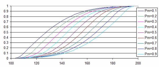
34. The
illustration below shows Cumulative Humphreys Distribution curves for a range
of Pm’s.

35. The
example below illustrates the construction of the Humphreys Distribution with
the parameters:
|
N= |
100 |
|
M= |
130 |
|
X= |
200 |
36. The
first stage in the process is to calculate Pm.
|
Pm
= |
(M - N) |
|
|
(X - N) |
37.
Inserting the parameters this gives:
|
Pm
= |
(130 - 100) |
= 0.3 |
|
|
(200 - 100) |
|
38. The
next stage is to establish a reference probability scale. The intervals of this
scale will depend be governed by the total number of data values, but will be
generated by the sequence:
1/2N, 1/N + 1/2N, 2/N + 1/2N, 3/N + 1/2N,
….. (N-1)/N + 1/2N
39. If
the number of data values N = 100 then the reference probability sequence would
be:
|
0.005 |
|
0.015 |
|
0.025 |
|
0.035 |
|
" |
|
" |
|
" |
|
" |
|
0.995 |
40. In
order to calculate the data points it is necessary to remap the reference
probability sequence. The chart below illustrates the process.
41. The
reference probability scale is shown on the horizontal axis, while the
re-mapped scale is shown on the vertical axis. The Humphreys Distribution assumes
that the distribution either side of the Most Likely point (M) is in the form
of a normal distribution. The first part of the curve is covered by the range
from zero to Pm. To construct the curve it is necessary to re-map this range
from zero to 0.5 (the probability that at which the Mode occurs on a Normal
Distribution). Re-mapping on this section of the curve is achieved by the
formula:
For P < Pm Pr = 0.5P/Pm
Where:
Pr = the re-mapped probabilities
P = the values of the reference probability
sequence
Pm =
the cumulative probability corresponding to the Most Likely point (M),
calculated as shown above.
42. The
second part of the curve is a little more difficult, but the process can be
followed by reference to the illustration above. The re-mapped probabilities in
the second part of the curve begin at a value of Pr = 0.5, so this is the first term in the
equation. In order to re-map the values of P, which lie above Pm, it is
necessary to deduct the value of Pm and then to adjust the proportions by
multiplying by 0.5 and dividing by (1 – Pm). The equation for the upper part of
the curve is shown below:
For P > Pm Pr = 0.5 + 0.5
(P – Pm)/(1 – Pm)
43. A
sequence of data is shown below. Although the value of P = Pm = 0.5 does not
appear in the reference probability sequence, it can be seen that, such a value
would correspond to a Pr value of Pr =
0.5.
|
P |
Pr |
|
0.005 |
0.0083 |
|
0.015 |
0.0250 |
|
0.025 |
0.0417 |
|
0.035 |
0.0583 |
|
" |
" |
|
" |
" |
|
" |
" |
|
0.285 |
0.4750 |
|
0.295 |
0.4917 |
|
0.305 |
0.5036 |
|
0.315 |
0.5107 |
|
0.325 |
0.5179 |
|
" |
" |
|
" |
" |
|
0.965 |
0.9750 |
|
0.975 |
0.9821 |
|
0.985 |
0.9893 |
|
0.995 |
0.9964 |
44. The
next stage in the process is to calculate the Normal Standard Deviates
corresponding to the values of Pr. In Excel this can be achieved using the
function: =NORMSINV(B37) Where B37 refers to the column and rows
containing the values of Pr. A segment of the table is shown below:
|
P |
Pr |
SD |
|
0.005 |
0.0083 |
-2.39398 |
|
0.015 |
0.0250 |
-1.95996 |
|
0.025 |
0.0417 |
-1.73166 |
|
0.035 |
0.0583 |
-1.56892 |
|
" |
" |
" |
|
" |
" |
" |
|
" |
" |
" |
|
0.285 |
0.4750 |
-0.06271 |
|
0.295 |
0.4917 |
-0.02089 |
|
0.305 |
0.5036 |
0.008952 |
|
0.315 |
0.5107 |
0.02686 |
|
0.325 |
0.5179 |
0.044776 |
|
" |
" |
" |
|
" |
" |
" |
|
0.965 |
0.9750 |
1.959963 |
|
0.975 |
0.9821 |
2.100164 |
|
0.985 |
0.9893 |
2.300346 |
|
0.995 |
0.9964 |
2.690114 |
45. The
Humphreys Distribution assumes that the distance (M – N) = -3SD and the
distance (X – M) = +3SD. The conversion of the SD values into values of ‘X’ is
undertaken in two parts.
For P<Pm Y
= M + (M –
N) SD/3
And for P>Pm Y
= M + (X –
M) SD/3
|
P |
Pr |
SD |
Y |
|
0.005 |
0.0083 |
-2.39398 |
106.060 |
|
0.015 |
0.0250 |
-1.95996 |
110.400 |
|
0.025 |
0.0417 |
-1.73166 |
112.683 |
|
0.035 |
0.0583 |
-1.56892 |
114.311 |
|
" |
" |
" |
|
|
" |
" |
" |
|
|
" |
" |
" |
|
|
0.285 |
0.4750 |
-0.06271 |
129.373 |
|
0.295 |
0.4917 |
-0.02089 |
129.791 |
|
0.305 |
0.5036 |
0.008952 |
130.209 |
|
0.315 |
0.5107 |
0.02686 |
130.627 |
|
0.325 |
0.5179 |
0.044776 |
131.045 |
|
" |
" |
" |
|
|
" |
" |
" |
|
|
0.965 |
0.9750 |
1.959963 |
175.732 |
|
0.975 |
0.9821 |
2.100164 |
179.004 |
|
0.985 |
0.9893 |
2.300346 |
183.675 |
|
0.995 |
0.9964 |
2.690114 |
192.769 |
46. It
can be seen that the values of Y in the above table do not extend to N = 100
and X = 200 this is because the reference probability sequence contains only
one hundred values and hence the probabilities of 0.00135 and 0.99865 are not
covered. However, if a greater number of data points had been covered by the
reference probability sequence, say 10,000, then it is likely that values below
N = 100 and X = 200 would have been created.
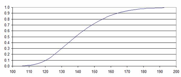
47. The
Cumulative Frequency Distribution for the Humphreys Distribution, with N = 100,
M = 130 and X = 200 obtained by plotting the values of P and Y from the above
data, is shown below:
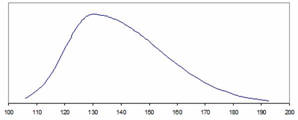
48. A
bell curve, useful only for illustration purposes, can be produced for this
data by utilising the Excel Function:
B =NORMDIST(M33,0,1,FALSE)
Where:
B = the ordinates of the
Bell Curve
M33 = Column and rows
containing the values of SD
0 = zero = the value of
the mean
1 = standard deviation =
1
False = to obtain the
bell curve rather than a cumulative frequency curve
The Bell Curve is then
obtained by plotting values of ‘Y’ against ‘B’
|
Y |
B |
|
106.0602 |
0.02272 |
|
110.4004 |
0.058445 |
|
112.6834 |
0.089076 |
|
" |
" |
|
129.7911 |
0.398855 |
|
130.2089 |
0.398926 |
|
130.6267 |
0.398798 |
|
131.0448 |
0.398543 |
|
" |
" |
|
179.0038 |
0.043968 |
|
183.6747 |
0.028305 |
|
192.7693 |
0.010702 |
ALTERNATIVE TO USING EXCEL FUNCTIONS
49. The example above demonstrated the use of
the Excel function =NORMSINV(Pr) to calculate a value of SD from Pr. It should
also be noted that Excel provides other useful functions such as = GAMMAINV(Po,
Alpha, Beta ) which will produce a cumulative Gamma distribution, = BETAINV(Po,
Alpha, Beta, Lower bound, Upper bound) which will produce a Beta distribution,
and LOGINV(Po, Mean, Standard deviation) which will produce a Lognormal
distribution, should these be required. The results of these Excel functions
are produced by an iterative process rather than by direct calculation.
50. Although the Excel library functions can be
used in an Access database, it may be found more convenient, and certainly
faster, to employ the equation set out below, which is shown in the “Handbook
of Mathematical Functions With Formulas, Graphs, and Mathematical Tables”
Edited by Milton Abramowitz and Irene A. Stegun published by the National
Bureau of Standards, United States Department of Commerce, Applied Mathematics
Series 55 June 1964. This equation only covers values of P up to 0.5 so a little manipulation is
necessary.
(P in the equation below is equal to Pr above)
THE
51. The
52. The graphs below illustrate the discrimination that this test
provides when fitting an NMX parameters of the Humphreys Distribution.

53. The graph above shows how the AD statistic
increases significantly if a small movement is made in the value of one of the
parameters, NMX, of the Humphreys distribution.
21. The figures in the graph above are based on the fitting of a
distribution where N = 18,800, M = 20,000 and X = 22,800. hence a
discrimination of +/- 5 is equivalent to
an accuracy of 2.5 x 10⁻⁴ .
54. The
a) The
data set comprising of ‘N’ data points (created using an Excel Beta Function
with parameters Alpha=9, Beta=5, Min=100, Max=200) is ranked in ascending order
as shown below. (the Rank column is used later so that data can be accessed as
a lookup table)
|
|
|
|
Rank |
Yi |
|
1 |
117.2852 |
|
2 |
119.7510 |
|
3 |
121.0388 |
|
4 |
121.9360 |
|
" |
" |
|
" |
" |
|
4998 |
164.9755 |
|
4999 |
164.9788 |
|
5000 |
164.9820 |
|
5001 |
164.9853 |
|
5002 |
164.9885 |
|
" |
" |
|
" |
" |
|
9997 |
194.7800 |
|
9998 |
195.1447 |
|
9999 |
195.6451 |
|
10000 |
196.5454 |
b) An estimate of the Humphreys Distribution
parameters is then made, in this case N=126.479, M=170.162, X=198.597 (which
gives a Pm of (170.162 – 126.479)/(198.597 – 126.479) = 0,60572) This is not a
particularly good fit, as shown in the illustration below, but it provides a
starting point. The data is shown in blue and the Humphreys Distribution
estimate is shown in red.

c) The next stage is to calculate the Standard
Deviates from the values in the data set, based on the assumed distribution.
The following equations are used for this operation:
For Yi < M
SD = 3(Yi – M)/(M – N)
And for Yi > M
SD = 3(Yi – M)/(X – M)
The results are as shown below:
|
|
|
Std Dev |
|
Rank |
Yi |
based on Yi |
|
1 |
117.2852 |
-3.6314 |
|
2 |
119.7510 |
-3.4621 |
|
3 |
121.0388 |
-3.3736 |
|
4 |
121.9360 |
-3.3120 |
|
" |
" |
" |
|
" |
" |
" |
|
4998 |
164.9755 |
-0.3562 |
|
4999 |
164.9788 |
-0.3560 |
|
5000 |
164.9820 |
-0.3557 |
|
5001 |
164.9853 |
-0.3555 |
|
5002 |
164.9885 |
-0.3553 |
|
" |
" |
" |
|
" |
" |
" |
|
9997 |
194.7800 |
2.5973 |
|
9998 |
195.1447 |
2.6358 |
|
9999 |
195.6451 |
2.6886 |
|
10000 |
196.5454 |
2.7835 |
b) The next stage is to calculate the
Cumulative Probabilities associated with each of these Standard Deviation
values. Because the two parts of the Humphreys Distribution are based on Normal
Distributions with different parameters, It is necessary to divide the
calculations into two parts. The formula are as follows:
For Yi < M Pi = NORMSDIST(SD) x Pm / 0.5
For Yi > M Pi =
Pm + (NORMSDIST(SD) – 0.5) x (1 – Pm) / 0.5
Values are produced as follows:
|
|
|
Std Dev |
Pi for |
|
Rank |
Yi |
based on Yi |
NMX Fit |
|
1 |
117.2852 |
-3.6314 |
0.000171 |
|
2 |
119.7510 |
-3.4621 |
0.000325 |
|
3 |
121.0388 |
-3.3736 |
0.000449 |
|
4 |
121.9360 |
-3.3120 |
0.000561 |
|
" |
" |
" |
" |
|
" |
" |
" |
" |
|
4998 |
164.9755 |
-0.3562 |
0.437145 |
|
4999 |
164.9788 |
-0.3560 |
0.437246 |
|
5000 |
164.9820 |
-0.3557 |
0.437347 |
|
5001 |
164.9853 |
-0.3555 |
0.437448 |
|
5002 |
164.9885 |
-0.3553 |
0.437550 |
|
" |
" |
" |
" |
|
" |
" |
" |
" |
|
9997 |
194.7800 |
2.5973 |
0.996295 |
|
9998 |
195.1447 |
2.6358 |
0.996690 |
|
9999 |
195.6451 |
2.6886 |
0.997171 |
|
10000 |
196.5454 |
2.7835 |
0.997880 |
55. Note
that the logic behind the Anderson Darling Test is not entirely clear (personal
comment – meaning that the author does not understand why it works), but
appears to be related to the fact that if the cumulative probabilities of the
data and the fitted distribution are plotted against each other, then if the
assumed distributions fits the data exactly, then the resultant plot will be a
straight line. The relevant plot is shown below:
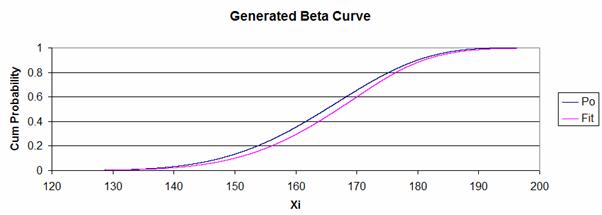
56. The
plot of Pi against PO is shown in red, while a straight line has been added in
black to demonstrate how the linear requirement is not met by the parameters
selected in the example. Note that the values of PO have been calculated by the
Rank sequence and are in the form:
1/2N, 1/N + 1/2N, 2/N + 1/2N, 3/N + 1/2N,
….. (N-1)/N + 1/2N
Where N = the number of data elements (this process is described in
section 38)
c) The next stages in the process are to
calculate the natural logarithms of Pi and (1 – Pi) these are shown below:
|
|
|
Std Dev |
Pi for |
|
|
|
Rank |
Yi |
based on Yi |
NMX Fit |
Ln(Pi) |
Ln(1-Pi) |
|
1 |
117.2852 |
-3.6314 |
0.000171 |
-8.675105 |
-0.000171 |
|
2 |
119.7510 |
-3.4621 |
0.000325 |
-8.032430 |
-0.000325 |
|
3 |
121.0388 |
-3.3736 |
0.000449 |
-7.707516 |
-0.000450 |
|
4 |
121.9360 |
-3.3120 |
0.000561 |
-7.485499 |
-0.000561 |
|
" |
" |
" |
" |
" |
" |
|
" |
" |
" |
" |
" |
" |
|
4998 |
164.9755 |
-0.3562 |
0.437145 |
-0.827491 |
-0.574732 |
|
4999 |
164.9788 |
-0.3560 |
0.437246 |
-0.827259 |
-0.574913 |
|
5000 |
164.9820 |
-0.3557 |
0.437347 |
-0.827028 |
-0.575092 |
|
5001 |
164.9853 |
-0.3555 |
0.437448 |
-0.826797 |
-0.575272 |
|
5002 |
164.9885 |
-0.3553 |
0.437550 |
-0.826565 |
-0.575453 |
|
" |
" |
" |
" |
" |
" |
|
" |
" |
" |
" |
" |
" |
|
9997 |
194.7800 |
2.5973 |
0.996295 |
-0.003712 |
-5.598116 |
|
9998 |
195.1447 |
2.6358 |
0.996690 |
-0.003315 |
-5.710816 |
|
9999 |
195.6451 |
2.6886 |
0.997171 |
-0.002833 |
-5.867693 |
|
10000 |
196.5454 |
2.7835 |
0.997880 |
-0.002122 |
-6.156329 |
d) The values of Ln(1 –Pi) are then reversed, such the
associated with the first element of data (the one which has the lowest value
in the set) there is the value of Ln(Pi) and set along-side, the value taken
from the last data element for Ln(1 – Pi) as shown below.
|
|
|
Pi for |
|
|
Reverse |
in reverse |
|
Rank |
Yi |
NMX Fit |
Ln(Pi) |
Ln(1-Pi) |
Rank |
Order |
|
1 |
117.2852 |
0.000171 |
-8.675105 |
-0.000171 |
10000 |
-6.156329 |
|
2 |
119.7510 |
0.000325 |
-8.032430 |
-0.000325 |
9999 |
-5.867693 |
|
3 |
121.0388 |
0.000449 |
-7.707516 |
-0.000450 |
9998 |
-5.710816 |
|
4 |
121.9360 |
0.000561 |
-7.485499 |
-0.000561 |
9997 |
-5.598116 |
|
" |
" |
" |
" |
" |
" |
" |
|
" |
" |
" |
" |
" |
" |
" |
|
4998 |
164.9755 |
0.437145 |
-0.827491 |
-0.574732 |
5003 |
-0.575632 |
|
4999 |
164.9788 |
0.437246 |
-0.827259 |
-0.574913 |
5002 |
-0.575453 |
|
5000 |
164.9820 |
0.437347 |
-0.827028 |
-0.575092 |
5001 |
-0.575272 |
|
5001 |
164.9853 |
0.437448 |
-0.826797 |
-0.575272 |
5000 |
-0.575092 |
|
5002 |
164.9885 |
0.437550 |
-0.826565 |
-0.575453 |
4999 |
-0.574913 |
|
" |
" |
" |
" |
" |
" |
" |
|
" |
" |
" |
" |
" |
" |
" |
|
9997 |
194.7800 |
0.996295 |
-0.003712 |
-5.598116 |
4 |
-0.000561 |
|
9998 |
195.1447 |
0.996690 |
-0.003315 |
-5.710816 |
3 |
-0.000450 |
|
9999 |
195.6451 |
0.997171 |
-0.002833 |
-5.867693 |
2 |
-0.000325 |
|
10000 |
196.5454 |
0.997880 |
-0.002122 |
-6.156329 |
1 |
-0.000171 |
In the last column it can be seen that the
value of -6.156329 which appears as the Ln(1-Pi) for item 10000 is now
associated with the first item.
e) An elemental statistic is then calculated,
for each row, by adding the values Ln(Pi) and ‘Ln(1 – Pi) in reverse Order’ and
multiplying this line sub-total by (1 – 2i)/N (where i = Rank)
|
|
|
Ln(1-Pi) |
|
|
|
|
in reverse |
|
|
Rank |
Ln(Pi) |
Order |
AD Stati |
|
1 |
-8.675105 |
-6.156329 |
0.001483 |
|
2 |
-8.032430 |
-5.867693 |
0.004170 |
|
3 |
-7.707516 |
-5.710816 |
0.006709 |
|
4 |
-7.485499 |
-5.598116 |
0.009159 |
|
" |
" |
" |
" |
|
" |
" |
" |
" |
|
4998 |
-0.827491 |
-0.575632 |
1.402422 |
|
4999 |
-0.827259 |
-0.575453 |
1.402291 |
|
5000 |
-0.827028 |
-0.575272 |
1.402161 |
|
5001 |
-0.826797 |
-0.575092 |
1.402029 |
|
5002 |
-0.826565 |
-0.574913 |
1.401898 |
|
" |
" |
" |
" |
|
" |
" |
" |
" |
|
9997 |
-0.003712 |
-0.000561 |
0.008543 |
|
9998 |
-0.003315 |
-0.000450 |
0.007528 |
|
9999 |
-0.002833 |
-0.000325 |
0.006315 |
|
10000 |
-0.002122 |
-0.000171 |
0.004586 |
The calculation for the fourth element is as
follows:
AD Stat(N=4) = (Ln(Pi) – ‘Ln(1-Pi)in
reverse’)(1 – (2Rank)/N
AD Stat(N=4) =
(-7.485499 -5.598116) ( 1 – (2 x 4))/10000
AD Stat(N=4) = ( - 13.083616 )( - 7)/10000 = 0.009159
f) The elemental statistics are then summed,
and ‘N’ deducted from the total, to produce the Anderson Darling Statistic
(AD).
|
|
|
Ln(1-Pi) |
|
|
|
|
in reverse |
|
|
Rank |
Ln(Pi) |
Order |
AD Stati |
|
1 |
-8.675105 |
-6.156329 |
0.001483 |
|
2 |
-8.032430 |
-5.867693 |
0.004170 |
|
3 |
-7.707516 |
-5.710816 |
0.006709 |
|
4 |
-7.485499 |
-5.598116 |
0.009159 |
|
" |
" |
" |
" |
|
" |
" |
" |
" |
|
4998 |
-0.827491 |
-0.575632 |
1.402422 |
|
4999 |
-0.827259 |
-0.575453 |
1.402291 |
|
5000 |
-0.827028 |
-0.575272 |
1.402161 |
|
5001 |
-0.826797 |
-0.575092 |
1.402029 |
|
5002 |
-0.826565 |
-0.574913 |
1.401898 |
|
" |
" |
" |
" |
|
" |
" |
" |
" |
|
9997 |
-0.003712 |
-0.000561 |
0.008543 |
|
9998 |
-0.003315 |
-0.000450 |
0.007528 |
|
9999 |
-0.002833 |
-0.000325 |
0.006315 |
|
10000 |
-0.002122 |
-0.000171 |
0.004586 |
|
|
|
Sum |
10,108.08 |
AD = Sum of elements – N = 10,108.08 – 10,000 =
108.08
An AD of 108.08 indicates that the distribution
selected, of N=126.479, M=170.162, X=198.597 does not fit the data.

.
57. It should be noted that with a normal distribution the points P = 0
and P = 1 correspond to + and – infinity. In creating a data it has been
assumed that values of Pi will be selected from the equivalent mid class
points, as such the values of Pi selected correspond to the series: 0.5/n,
0.5/n + 1/n, 0.5/n + 2/n, …..etc. where n equals the number of data points to
be selected. For n = 10,000 the series would be of the form 0.00005, 0.00015,
0.00025, etc upto 0.99995
58. It should also be noted that it is assumed value of N and X occur at
-3 and +3 standard deviations, corresponding to probabilities of 0.00135 and
0.99865. From the above it will be apparent that a number of the values in the
data set will lie outside the N and X limits.
REFERENCES
Humphreys G. (1979) Turning Uncertainty to Advantage, McGraw-Hill Book Company (UK) Limited. P22-30