Squaring a Normal Distributions

By P Barber (March 2010)

(Back)

Abstract

This paper develops a set of empirical equations for calculating the Humphreys distribution parameters of a dataset obtained by squaring a Humphreys distribution with Pm = 0.5. (Where a Humphreys distribution with Pm = 0.5 represents a set with a Normal distribution)

Introduction

1. The parameters of a Statistical Distribution provide a precise definition of a dataset. If two Statistical Distributions are multiplied together, the result will also be precisely defined.

2. This paper examines the effect of squaring normal distributions with varying tolerance T.

Where T = 0.1 in combination with a Mean Value (Mi) of 20,000 would provide a three standard deviation limit of 0.1 x 20,000 = +/- 2,000,

Or a Humphreys distribution with factors: Mi = 20,000, Ni = 18,000 (20,000 – 2,000) and Xi = 22,000 (20,000 + 2,000). With Pm = (Mi – Ni) / (Xi – Ni) = 2,000/4,000 = 0.5

By definition any Humphreys distribution with Pm = 0.5 is a normal distribution with Standard deviation = (Xi – Ni)/6 = 4,000/6 = 666.66666^.

3. The table below shows the results of a series of tests which indicate the effect of squaring Normal distributions with differing tolerances.  The data in the table has been determined by fitting a Humphreys distribution to the results of a Monte Carlo simulation, using the Anderson Darling technique. The Anderson Darling statistic is shown along side each of the fitted results.

Based on M2 = 400,000,000
T	No	Mo	Xo	AD
0.05	371,438,028	400,020,308	428,537,578	0.147249
0.10	344,136,500	399,068,200	457,469,800	0.171935
0.15	315,828,356	398,368,686	487,064,901	0.138283
0.20	290,512,955	396,182,227	516,002,564	0.287446
0.25	264,877,424	393,154,505	546,871,229	0.121250
0.30	238,407,582	390,492,388	578,003,027	0.165118
0.35	213,249,882	386,961,332	609,257,224	0.173640
0.40	188,606,512	382,883,310	640,941,171	0.189685
0.45	164,480,277	378,263,005	673,044,064	0.209646
0.50	139,859,418	374,094,343	704,628,005	0.249577
0.55	117,682,172	368,828,250	735,650,020	0.503540
0.60	95,220,720	361,198,110	771,765,200	0.296411
0.65	73,866,500	356,232,000	801,269,800	0.677293

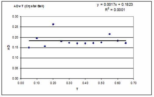
4. It was noted that the software pckage Oracle Crystal Ball indicated that it was possible to fit a Gamma distribution to many of the results of the Monte Carlo distribution. For T = 0.6 a Gamma distribution was fitted with AD = 0.1824 however for T =0.65 the best fit was a Lognormal distribution with AD = 0.1715

T	Crystal Ball Best-Fit	AD
0.05	Normal	0.1502
0.10	Gamma	0.1961
0.15	Gamma	0.1563
0.20	Gamma	0.2634
0.25	Gamma	0.1802
0.30	Gamma	0.1739
0.35	Gamma	0.1701
0.40	Gamma	0.1705
0.45	Gamma	0.1719
0.50	Gamma	0.1751
0.55	Gamma	0.2166
0.60	Gamma	0.1824
0.65	Log Normal	0.1715

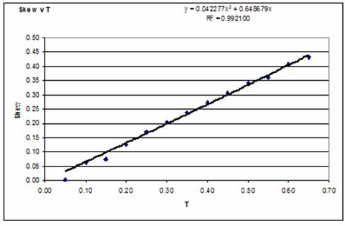
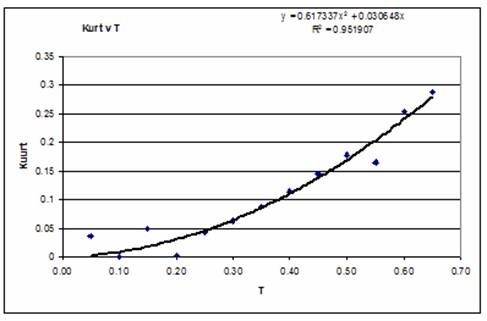
5.  In the graph below the values of AD shown in the table are plotted against the tolerance  T, and a trend line added as a reference. While it is considered that the trend line has little if any significance, it can be seen that a number of points, namely those at T = 0.05, 0.15, 0.20 and 0.55 appear at a significant distance from the trend line, it is postulated that these data points have been derived from distributions which are less representative. It will also be noted that these data points deviate from the trend line on the curves plotted for Skew v T and for Kurt v T, which are shown in the appendix. It should be noted however, that these points appear to have little effect (other than the AD Statistic) on the factors calculated for the Humphreys distribution parameters.

6.  In the table below the No.Mo.Xo parameters of the Humphreys distribution have been converted into normalised factors, by dividing the parameters by Mi² (in this case Mi2 = 400,000). The table also shows the Skew, Kurt and the Ratio ‘Standard deviation/Average’ for the distributions produced.

T	Fn	Fm	Fx	Skew	Kurt	Std/Ave
0.05	0.928595	1.000051	1.071344	0.002556	0.037161	0.023813
0.10	0.860341	0.997671	1.143675	0.064519	0.000399	0.047153
0.15	0.789571	0.995922	1.217662	0.075656	0.049689	0.071436
0.20	0.726282	0.990456	1.290006	0.126011	0.003346	0.094078
0.25	0.662194	0.982886	1.367178	0.169637	0.042688	0.118037
0.30	0.596019	0.976231	1.445008	0.204375	0.063460	0.141746
0.35	0.533125	0.967403	1.523143	0.238892	0.087514	0.165512
0.40	0.471516	0.957208	1.602353	0.273145	0.114802	0.189343
0.45	0.411201	0.945658	1.682610	0.307096	0.145272	0.213251
0.50	0.349649	0.935236	1.761570	0.340703	0.178862	0.237244
0.55	0.294205	0.922071	1.839125	0.360889	0.165086	0.260417
0.60	0.238052	0.902995	1.929413	0.406735	0.255123	0.285525
0.65	0.184666	0.890580	2.003175	0.432517	0.287410	0.309104

7. Plotting the factors Fn, Fm, Fx against T, and fitting a line reveals that a reasonable trend-line can be developed for each of the factors and the fitted equations provide the basis for the empirical relationship. Note that the trend line was forced to pass through the point T = 0, F(n,m,x) = 1.000, because if T = 0, then both input and output variables are represented by single numbers such that:

No = Mo = Xo = Mi².

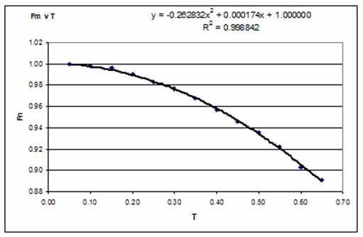
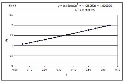
8. The fitted trend lines provide the following empirical equations for estimating the values of Fn, Fm and Fx:

Fn =	0.260265 T^2   -   1.425717 T   +   1.000
Fm =	0.262832 T^2   +   0.000174 T   +   1.000
Fx =	0.190183 T^2   +   1.426252 T   +   1.000

Example

9. Given the parameters of a symmetrically distributed Humphreys distribution:

Ni =	18,000
Mi =	20,000
Xi =	22,000

It is first necessary to calculate the value of Pm, to ensure that Pm = 0.5

Pm = (Mi – Ni)/(Xi –Ni) = (20,000 – 18,000)/(22,000 – 18.000) = 0.5 indicating that the condition is satisfied.

The value of T = (Xi – Ni)/(2 x Mi) = (22,000 – 18,000)/( 2 x 20,000) = 0.1

	T^2 = 0.001	T = 0.1	Plus 1
Fn constants	0.260265	-1.425717	1.000000
Fm constants	0.262832	0.000174	1.000000
Fx constants	0.190183	1.426252	1.000000
Multiply by:	T^2 = 0.001	T = 0.1	Plus 1	Total
Fn =	0.002603	-0.142572	1.000000	0.860031
Fm =	0.002628	0.000017	1.000000	1.002646
Fx =	0.001902	0.142625	1.000000	1.144527
Mi^2 =				400,000,000
Multiplying Fn, Fm and Fx by Mi^2 yields:
No =				344,012,380
Mo =				401,058,288
Xo =				457,810,812

Conclusion

10. It can be seen from the above that it is possible to generate a meaningful parametric relationship for determining the Humphreys distribution parameters for the results obtained by squaring a Normal distribution. However, a number of questions remain. First is the question of accuracy. The empirical relationships described above have been based on single point results. It is also recognised that the distribution produced by a Monte Carlo Simulation is not smooth and is not repeatable. It seems likely however, that utilising the results of many simulations would enable the Humphreys distribution parameters to be fitted with accuracy. Although it is apparent from the analysis above that the Humphreys distribution does not provide a good fit, as the Tolerance T of the input distribution is increased. However, the value of AD is not sufficiently high to reject the Null Hypothesis, that the results could not have been drawn at random from a Humphreys distribution. In support of this assertion the graph below shows the results of a series of a series (100) of simulations designed to determine the significance level of associated with the final result No = 73,866,500 Mo = 356,232,000 and Xo = 801,269,800. (Pm = 0.38818)

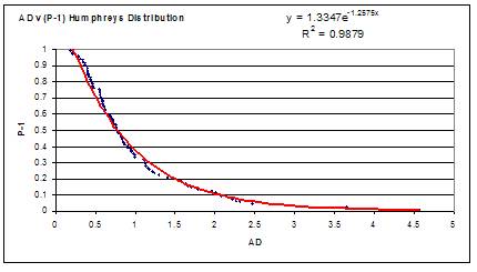
11. Referring to the above graph, at the AD of 0.677293 associated with the last result, the level of significance is approximately 60%, which is quite high since it is usual to reject at the 0.05 level, which corresponds to AD values greater than about 2.4. Hence it can be claimed that the Humphreys distribution provides a good fit of the results of squaring normal distributions, at least up to T = 0.65

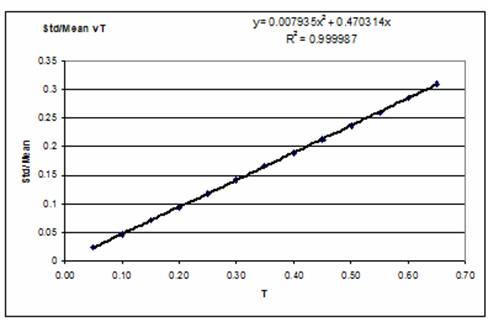
Appendix

This appendix shows plots of parameters derived using Excel functions from the datasets, of N = 10,000 values produced by Monte Carlo simulation. The plots are:

a) Skew v T

b) Kurt v T, and

c) Std/Average