Re-examination
of Sales Price & Volume Variance
by P Barber
Introduction
1. This paper takes a
fresh look at the process of Sales Price and Volume Variance
Analysis and concludes that “Mix” provides an unsatisfactory explanation
of the difference often found between High-Level and Detail-Level
calculations, that this difference is driven by the combination of elements
with significantly different sales prices being included within a single data
set, and that the correct separation of Total Sales Variance into its
Price and Volume related components is achieved by adding the detail, rather
than drilling down into the data from the top level.
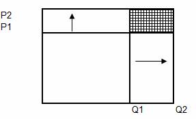
This process is
illustrated graphically to demonstrate the issues involved. The area of the
diagram below represents Sales Income in period 1.
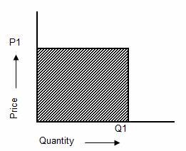
Where:
P1 = Sales price-each
in period 1
Q1 = Quantity sold in
the period 1
The area of the shaded
portion = P1 x Q1 = Sales Income in period 1 = S1
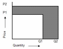
Where:
P2 = Sales price-each in period 2
Q2 = Quantity sold in the period 2
S2 = Income in period 2 = P2 x Q2
3. The shaded area
indicates the change in income (S2 – S1) = (P2 x Q2) – (P1 x Q1)
The challenge in Sales
Price and Volume Variance Analysis is to divide this shade area into its
Price related and Volume related elements.
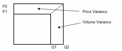
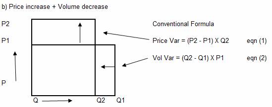
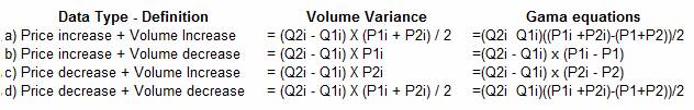
4. The traditional set
of formula (Anthony 1970) used for this application are shown below:

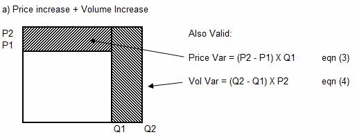
5. However, this is
not the only way in which these variances can be defined, Anthony (1970) states
that the following analysis is also valid.
6. Yet another way in
which the variance can be allocated is by treating each element as a trapezium,
as shown below.
7. The area of a
trapezium is given by the equation:
Area of Trapezium = Width x Average Height.
Therefore the
equations for Price and Volume Variance become:
Price Variance = (P2
–P1) x (Q2 + Q1) / 2 eqn (5)
Volume Variance = (Q2 –
Q1) x (P2 + P1) / 2 eqn (6)
8. Each of the three
sets equations (eqn 1 to 6) illustrated above are valid for situations when either both the Price
and the Volume increase from period 1 to period 2, or alternatively, when both
Price and Volume decrease between period 1 and period 2. The difference between
the alternative equations relate to the way in which the corner (shown shaded)
is divided between the two Variances.
9. The extreme
positions are represented by the equations which either place the whole of the
shaded area as Volume Variance (eqns 3 & 4), or the whole of the
shaded area as Price Variance (eqns 1 & 2). There is an equal probability of the Price and Volume Variances
being any value between the two extremes. If individual elements of a data-set
were to be summed across the whole set then the final result would be equal to
the median value between these two extremes. The geometric equations shown
above (eqns 5 & 6) allocate the variance in the same way, allocating
the shaded portion equally between the two extremes.
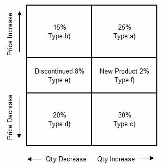
10. For convenience,
in this paper, the situation where both price and volume increase between
periods 1 and 2 are referred to as “type a)” while the situation where both
price and quantity decrease between periods 1 and 2 are referred to as “type
d)”. Equations (5) and (6) are
appropriate to both of these situations.
11. The conventional
formula is appropriate to situations where the price-each increases
between period 1 and period 2, while the quantity is reduced. This situation,
referred to in this paper as “type b)”, is illustrated below:
12. The conventional
formula does not however fit the situation where price-each reduces, between
periods 1 and 2, while quantity increases. This situation, referred to in this
paper as “type c)” is shown below:
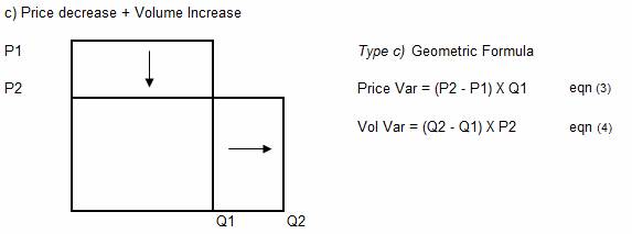
13. It can be seen
that the “geometry” for types b) and type c) is similar. However,
parts of the equation have been swapped, with P2 replacing P1 in the Volume Variance
equation and Q1 replacing Q2 in the Price Variance equation.
Type e) Q2 = 0, Q1 > 0
Type f) Q1 = 0, Q2 > 0
Type g) Q2 = 0, S2 <> 0
Type h) Q1 = 0, S1 <> 0
Type e) is a discontinued product, while type f)
is a new product. With both types e) and type f) all of the Sales
Income change is attributable to a change in volume, the whole of the
variance (S2 – S1) is therefore allocated as Volume Variance.
Types g) and type h) involve value only
credit-notes and here all the Sales Income change should be allocated as Price
Variance.
15. It should be noted
that (Price Variance + Volume Variance) = Total Variance =
(S2 – S1). This fact means that in a study of Price and Volume Variance
it is only necessary to study one of the variances: either Price Variance,
or Volume Variance. For practical calculation the author prefers to
calculate Price Variance by backing out from the total Variance:
Price Variance = (S2 – S1 – Volume
Variance )
16. The table below
illustrates the Volume Variance calculated using each of the equations
on a constant type a) data set.
|
a) Price increase +
Volume Increase |
|
|
|
|
|
|
|
|
|
Type |
Volume Variance Equation |
Q2 |
Q1 |
P2 |
P1 |
S2 |
S1 |
Vol Var |
|
a |
= (Q2 - Q1) X (P1 + P2) /
2 |
30 |
20 |
7 |
2 |
210 |
40 |
45 |
|
b |
= (Q2 - Q1) X P1 |
30 |
20 |
7 |
2 |
210 |
40 |
20 |
|
c |
= (Q2 - Q1) X P2 |
30 |
20 |
7 |
2 |
210 |
40 |
70 |
|
d |
= (Q2 - Q1) X (P1 + P2) /
2 |
30 |
20 |
7 |
2 |
210 |
40 |
45 |
It can be seen that
the values calculated using the type a) and type d) methods (eqns
5 & 6) are identical, while the values calculated using the type b) and
the type c) methods are significantly different from the values
calculated using the type a) and type
d). The type b) and type c) methods show the extremes of the
possible values, while type a) and type d) methods show the
average of type b) and type c) methods. That is: (20 + 70)/2 =
45. It can be seen that failure to use the correct formula will result in
significant analytical errors.
Difference between
Detail and High-Level Calculations
18. When performing
Price and Volume Variance Analysis on a set of data it is often found that the sum
of the elemental Price and Volume Variances do not add up to the values
calculated at the total level. The example below, which uses the traditional
equations (eqns 1 & 2) illustrates the point:
|
a) Detail Calculation |
|
|
|
|
|
|
|
|
|
|
Set |
Q2i |
Q1i |
P2i |
P1i |
S2i |
S1i |
VolVari |
PriceVar |
Total |
|
A |
100 |
80 |
5 |
3 |
500 |
240 |
60 |
200 |
260 |
|
B |
200 |
40 |
8 |
6 |
1600 |
240 |
960 |
400 |
1360 |
|
|
300 |
120 |
|
|
2100 |
480 |
1020 |
600 |
1620 |
|
|
|
|
|
|
|
|
|
|
|
|
b) High Level Calculation |
|
|
|
|
|
|
|
| |
|
|
Q2 |
Q1 |
P2 |
P1 |
S2 |
S1 |
VolVar |
PriceVar |
Total |
|
Total |
300 |
120 |
7 |
4 |
2100 |
480 |
720 |
900 |
1620 |
The nomenclature used in the example above is as
follows:
Q1i = Quantity sold in period 1 for each element i
Q2i = Quantity sold in period 2 for each element i
P1i = Price-each for each element in period 1. (at total
level = sum(S1i)/sum(Q1i)
P2i = Price-each for each element in period 2. (at total
level = sum(S2i)/sum(Q2i)
S1i = Income from each element i, in period 1 = Q1i x P1i
S2i = Income from each element period 2 = Q2i x P2i
VolVar i = Volume Variance = (Q2i – Q2i) x P1i
PriceVar i = Price Variance = (P2i – P1i) x P2i
Q1 = S Q1i = the sum of the elemental Quantities for period 1
S = the mathematical symbol meaning the sum of all the
values i = 1 to n
n = number of values in the set
Q2 = S Q2i = the sum of the elemental Quantities for period 2
S1 = S S1i = the sum of the elemental Sales Income for period
1
S2 = S S2i = the sum of the elemental Sales Income for period
2
P1 = S1 / Q1 = Average price-each for the total set in
period 1
P2 = S2 / Q2 = Average price-each for the total set in
period 2
VolVar = Volume Variance = (Q2 – Q2) x P1
PriceVar = Price Variance = (P2 – P1) x P2
In the example it can be seen that the sum of the Volume Variance in the first calculation is 1020 and
the sum of the Price Variance is 600. However, the
Volume Variance calculated at the Total level is 720
and the Price variance
The example demonstrates that the level of analysis has the
effect of swapping a “piece” of the Variance between Volume and Price columns. The
difference between the two calculations (VolVar: 1020 – 720 = 300) and
(PriceVar: 600 – 900 = -300) has traditionally (Anthony 1970) been referred to
as Mix.
This difference, also referred to as “Consolidation Adjustment” in this paper, raises a
number of questions, including:
a) What is the reason for this difference and how can it be
explained?
b) What equations can be used to explain this difference?
c) Does this difference represent a separate Variance, or does
it operate as an equal and opposite adjustment to the Price and Volume Variance
total-columns?
d) Which answer is correct, the High-Level Calculation or the sum of the Detail-Level Calculations?
e) Can parts of this difference be assigned to individual
detailed elements, or does this difference only exist at the High-Level?
f)
What steps can be taken to minimise this difference?
In order to answer these questions I would like to start
with question e)
Can the Difference be
assigned to individual detailed elements?
19. To answer this question the author conducted an
experiment in which elements of data were changed and the resultant movement in
Volume Variance, at the High-Level, was recorded.
It is argued that if a specific change at the detailed
level results in a consistent movement in the Volume
Variance, recorded at the high level, regardless of the condition of other
elements in the data set, then parts of the difference can be specifically
assigned to an individual detailed element.
The following assumptions were made during this
experiment:
a) That the traditional formulas for Price and Volume Variance would be used (eqns
1 & 2)
b) That the elemental data for period 1 would remain fixed.
This seemed a reasonable assumption since all the data for period 1 would be
known and would not be subject to amendment as a result of information received
following the end of period 2.
The initial data set for this experiment is shown
below:
|
Initial Data Set: |
|
|
| ||||
|
Data Set |
Q2i |
Q1i |
P2i |
P1i | |||
|
A |
100 |
100 |
8 |
8 | |||
|
B |
50 |
50 |
10 |
10 | |||
|
C |
200 |
200 |
12 |
12 | |||
While the final state of each of the data elements is given
by:
|
Final Data Set: |
|
|
| ||||
|
Data Set |
Q2i |
Q1i |
P2i |
P1i | |||
|
A |
80 |
100 |
10 |
8 | |||
|
B |
45 |
50 |
12 |
10 | |||
|
C |
180 |
200 |
14 |
12 | |||
The sequences in which these elements of data can be
changed are set out in the table below:
|
Test1 |
Test 2 |
Test 3 |
Test 4 |
|
A |
B |
B |
C |
|
|
A |
C |
A |
|
|
|
A |
|
The tabular calculation below shows the Detailed and High-Level
calculations for the initial state.
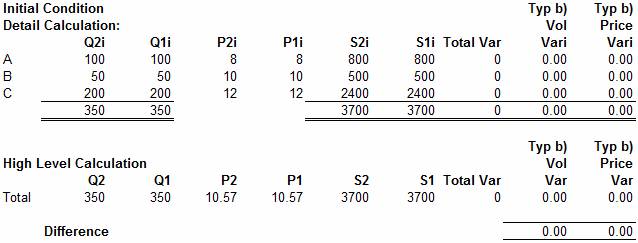
With the elemental quantities: Q2i = Q1i and elemental
prices: P2i = P1i, it can be seen that the elemental Volume and Price Variances equal zero:
VolVari = (Q2i –
Q1i)P1i = zero
PriceVari = (P2i – P1i)Q2i =zero
The same result is found with the High-Level calculation, which is based on the sum of
the low level quantities:
Q1 = S Q1i and Q2 = S Q2i
and the average prices:
P1 = S (Q1i x P1i) / S Q1i = 3700 / 350 = 10.57
P2 = S (Q2i x P2i) / S Q2i = 3700 /350 = 10.57
With Q2 = Q1 and P2 = P1 the High-Level Price
and Volume Variances are also equal to zero:
VolVar = (Q2 – Q1)P1 =
zero
PriceVar= (P2 – P1)Q2 = zero
In the first test the details for element “A” are changed
and the High-Level change in Price and Volume Variance is measured, between the
initial state (zero as shown above) and this new result. The calculation is
shown below:
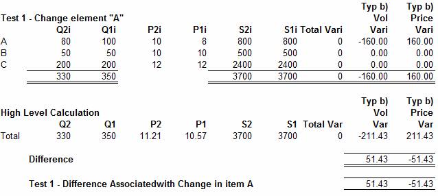
Hence it can be seen that the change to the data of element
“A” has caused a difference (Consolidation Adjustment) of 51.43 to the Volume
Variance and -51.43 to the Price Variance Column.
In Test 2 we begin with a data set where the value of
element “B” has been changed and monitor the change in “Consolidation Adjustment” when element “A” is then
changed. This is shown in the calculation below:
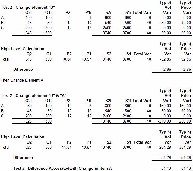
As can be seen the change of 51.43 caused by the change in
element “A” is the same as in the first Test. The remainder of the Tests were
carried out, and in each case, [for type b) data, where price each increased
between periods 1 and period 2, while the quantity sold decreased between
periods 1 and period 2, using eqns (1) & (2)], the result was the same; confirming that a change in the
High-Level Price and Volume Variance can be associated with a change in an
individual line item. This association leads on to a consideration of the
equations proposed for explaining the difference between the High Level and
Detailed calculations.
20. The example above also demonstrates that the Difference
between the High and Detailed-Level calculations is
manifest, not as a separate variance which is measured in addition to Price and Volume Variance, but, as an equal and
opposite adjustment to the Price and Volume
Variance; having the effect of correcting the values calculated for both of
these variances. This is a useful conclusion as it means that the same equations
which account for the difference on one of the variances can also be applied to
the other.
Equations defining the
difference between High and Detail-level Calculations
21. Equations defining the difference between High and Detail-level calculations include:
a) The traditional equation, described as “mix” by Anthony
(1970), has the following form:
Mix = S ((Q2i – (R x Q1i)) x P1i )
eqn (7)
Where R = Q2/Q1 (the ratio of Quantity sold at the High Level, for periods 2 and 1)
b) An alternative equation, described by the author as “level adjustment” or “the Gama
adjustment” (ref 1) is as follows:
Gama = S ((Q2i – Q1i) x (P1i – P1))
eqn (8)
c) Another equation is:
Beta = S ((P1i – P1) x Q2i)
eqn (9)
d) It has been known for the difference between the High and Detailed-Level calculations to be apportioned
across the detailed elements using any available variable which was though to be
appropriate. Such variables could include: Q1i, Q2i, S1i, S2i, VolVari,
PriceVari, etc. The equation defining the elemental “Adjustment” in this case
would be of the form:
Alpha(V) = S (L x vi / V)
eqn
(10)
Where:
L = Level Adjustment: the difference between the High and
Detailed level calculations.
vi = Elemental value of
the variable selected: Q1i, Q2i, VolVari, PriceVari, etc.
V= Sum of the elemental values (vi) at the High Level: Q1,
Q2, VolVar, PriceVar, ETC.
It should be noted that the terms: Apha(V), Beta and Gama, have no context beyond their use in this paper,
as a means of reference, and should not be confused with their application in
other areas.
The difference in the results of these different
calculation methods, which refers only to differences in the calculation of Volume Variance (see 20. above), is illustrated in the
example below:
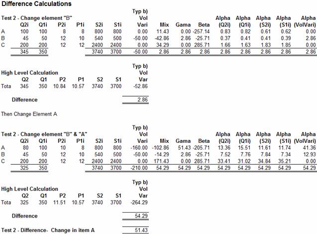
The example above is based on the data used in Test2,
illustrated in section
Here it can be seen that the Difference between the High
and Detailed Level calculations is found to be 2.86. This value is shown at the
bottom of the “Typ b) Vol Vari” and is the difference between the Sum of the
Volume Variances calculated at the detail level ( 0 – 50.0 – 0 = -50) and the
Volume Variance calculated at the High Level (345 – 350) x 10.57 = - 52.86);
with the difference being (- 50.0 - - 52.86 = 2.86)
It can be seen that each of the equations (Mix, Gama, Beta and Alph(v)
)
correctly
calculates the total difference. However, only the Gama and Alpa(VolVari)
equations correctly associate the whole of the difference to element “B”, the
only element which has changed. All the other equations spread parts of the
difference across all the other elements.
Examination of the results for the second part of the test,
where both elements “B” and “A” have been changed, reveals a similar pattern,
here it can be seen that all of the equations correctly calculate the total
Difference (-210 - - 264.29 = 54.29). However, only the Gama equation correctly states that the difference due
to element “B” is 2.86 and the Difference due to element “A” is 51.43.
The Alpha(VolVari) equation no
longer correctly associates the Difference to the appropriate element and all
the other equations allocate the Difference in some sort of manner in which the
author has struggled to provide a meaningful interpretation. Hence it is
concluded that, where type b) data is involved (Price increase combined with
Quantity decrease), the “Gama” equation correctly
assigns the Difference to those elements which drive that Difference.
What can the Gama equation
tell us about the Nature of the Difference
22. For convenience the Gama
equation is reproduced below:
Gama = S ((Q2i – Q1i) x (P1i – P1))
eqn (8)
If this equation is expanded into its component parts:
Gama = S ((Q2i – Q1i) x P1i) – S ((Q2i – Q1i) x P1)
The first term of the equation (A) is equal to the sum of
the elemental Volume Variances:
(A) Sum of elemental
Volume Variances = S ((Q2i – Q1i) x P1i)
While the second term (B) can be manipulated and expressed
in terms of Q2, Q1 and P1 and is found to be equal to the High-Level Volume Variance:
(B) High-Level Volume Variance = S ((Q2i – Q1i) P1 = (S(Q2i) – S (Q1i))P1 = (Q2 – Q1)P1
Hence it can be seen that the two components (A) and (B) of
the Gama equation merely state that the difference
between the High and Detailed calculations is due to
using last years’ average price as opposed to last years’ elemental price.
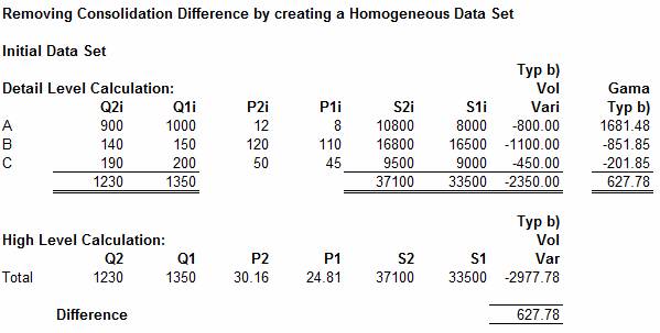
Difference caused by using
Average price-each as opposed to Elemental price each
23. Given that the Difference
is driven by the difference between the elemental and average price for the set,
it can be seen that, with reference to type b) data, the Difference reduces to zero if the data set is
homogeneous in regard to last years’ price each. It can be shown that this
principle can be extended to cover data types a) c) and d). This important
property is illustrated in the example below:
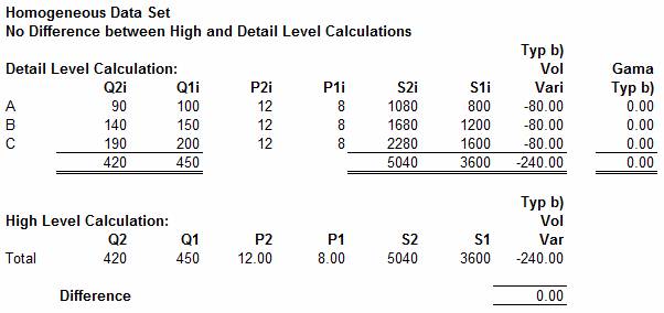
As can be seen, as a result of the re-mapping, the Difference in a homogeneous data set is reduced to
zero. This is a useful result as it enables the magnitude of the Difference to be reduced, by changing the counted
quantity. The argument goes like this: there is nothing sacrosanct about the
unit of Quantity-sold, or the price for that matter.
The Sales income in periods 1 and 2 (S1i and S2i) are fixed, although there
could be a change associated with the need to convert from one currency to
another. If a business sold nails, it could sell them by unit, by gross (144),
by 20, by 50, or by 1000, by kilo or pound (weight or sterling), the list of
counting units available is endless. Since the result of a mathematical
calculation should not be affected by the units of measure, it is concluded that
it is valid to adjust the Quantity-sold and Price-each of elements, to establish a homogeneous set
of data. The example below illustrates the principle:
Now suppose that we select a Sales
price-each for period 1 of 40 units each (in practice any value could have
been selected). Then we can restate the data shown above by adjusting the
Quantities and Prices to reflect this change. The re-mapping process applied to
element (A) is as follows:
Q2(A) = (Q2i x P1i / P1) = 900 x 8 / 40 = 180
Q1(A) = (Q1i x P1i / P1) = 1000 x 8 / 40 = 200
P2(A) = (P2i x P1 / P1i) = 12 x 40 / 8 = 60
P1(A) = (P1i x P1 / P1i) = 8 x 40 / 8 = 40 = P1
Where P1 = the value
selected for the Price-each in period
The other elements (B) and (C) are remapped in the same way to establish the data set
shown below:
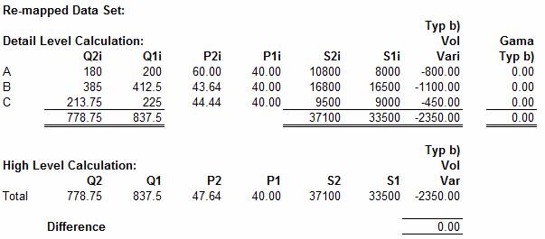
As can be seen, the effect of calculating the Volume Variance from the re-mapped data is to provide a
calculation at the High-Level which is free from “Consolidation Error”.
An important conclusion to be drawn from this analysis is
that the correct separation of the Total Sales
Variance into its Volume and Price related component parts can be achieved
by summing up the detailed elemental analysis.
Top-down or Bottom-up
24. Anthony (1970) regards the Difference between High and
Detailed-Level calculations to be due to “Mix”
and states that “the mix phenomenon arises whenever a cost or revenue is
analysed by component, rather than in total. If revenue is analysed by
individual products, or by individual geographic regions, a mix variance
inevitably arises. Failure to appreciate this fact can lead to great frustration
in trying to make the figures add-up properly.”
Anthony sees variance analysis as a tops-down process,
where the Analyst identifies a significant variance at the top-level, and then
drills-down into the data to determine the reason for the variance. Anthony
implies that the deeper the analyst drills the data the greater the amount of “mix” becomes.
Another feature of drilling data is that the data is
divided into smaller and smaller elements. There comes a point where it is no
longer possible to analyse the data, because time, product and customer
comparisons are no longer available, and it is therefore not possible to create
meaningful elemental sets as more data becomes classified as either a new
product: type f), or a discontinued product: type f) and more and more of the
data is classified as Volume Variance. Given the apparent
futility of drilling further and further into the data, in an attempt to find
“the correct answer” it is temping to regard the answer calculated at the High-Level to be the “correct answer”, and “Mix” to be an error, introduced by the Analyst as a
result of drilling the data.
25. However, the analysis above demonstrates
that the Difference between High and Detailed-Level calculations is caused by
combining data elements which have significantly different Sales prices. And it
is the significantly different Sales prices which cause a “Consolidation Error” to be created when calculations
are carried out at the High-Level. It is therefore
concluded that a correct separation of Sales Variance
into its respective Price and Volume Variance
components is best achieved by calculating from price-homogeneous elements and summing the
elemental variances to create the High-Level
Variances. However, in practice it is found that it is often not possible to
fully eliminate the effects of “Consoildation Error”
and it is therefore recommended that the “Gama
equation(s)” be used to identify the amount of error associated with individual
elements of the data set.
It should be noted that the original application of “Mix” (Anthony 1970) was to materials consumption, where
variances were measured against a standard. Mix
Variance applied to situations where the proportion of raw materials
deviated from standard. As such a separate and independent “Mix Variance” was created. “Sales Income Volume and Price Variance Analysis” does
not involve the use of a Standard and the use of the traditional “Mix” equation does not appear to be appropriate to this
application.
Data Analysis involving
all Data Types
The above analysis concentrated on type b) data, where
price each increases and quantity decreases between periods 1 and 2. The full
set of equations for each data type are shown below:
Where:
Price
Variance
= (Q2i x P2i) – (Q1i x P1i) – Volume Variance(i)
Q1i = elemental quantity sold in period 1
Q2i = elemental quantity sold in period 2
P1i = elemental price-each in period 1
P2i = elemental price-each in period 2
P1 = Average Price for the whole set in period 1
P2 = Average Price for the whole set in period 2
These equations are used in the example below which
incorporates all the main data types in a single calculation:
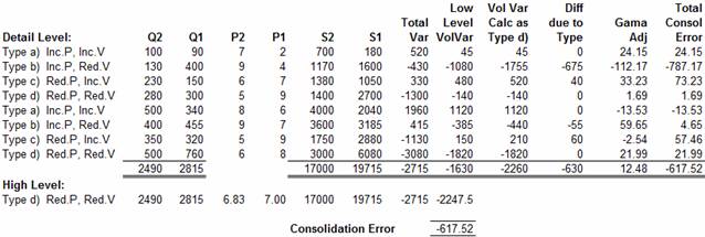
In the above example the total quantities and average
prices for the whole set are assessed and at the High-Level the set is found to be of type d). The
calculation of Volume variance (VolVar) is then
carried out using the equation appropriate to the elemental data type with the
results shown in the column headed “Low Level VolVar”. The Sum of the elemental
Volume Variances is equal to
minus 1630, while the Volume Variance calculated at the High-Level is equal to minus 2247.5. The difference
between these two numbers, the Consolidation Error, is equal to minus
617.52.
The next stage in the calculation is to calculate the
elemental Volume Variance using the equation
appropriate to the total set, in this case using the equations for type d),
since this was found to be the type for the total set. These calculations are
shown in the column headed “ Vol Var Calc as Type d)”, the sum of this column is
minus 2260
The difference between the two elemental Volume Variance calculations is shown in the column
headed “Diff due to Type”. The total of the column is equal to minus 630 (2260 -
1630)
The next column shows the Gama Adjustment appropriate to the High-Level data type, in this case type d), and the sum
of the column is equal to 12.48
The final column shows the sum of the “Diff due to Type”
and the “Gama Adjustment”, to reveal the elemental
“Total Consolidation Error”. The sum of the “Total Consolidation Error” is equal to minus 617.52
(12.48 – 630), the same value as shown at the bottom of the calculation, as the
difference between the High and Detail-Level
calculations.
It should be noted that correct value for the Volume Variance at the High-Level is minus 1630 and the correct Price Variance at the High-Level is minus 1085 (the Total Variance – Volume
Variance = (-2715 - - 1630) = 1085). The “Consolidation Error” is minus 617.52 and this is
relevant when trying to explain why the “High-Level”
calculations of Price and Volume Variance was not
correct.
About the Author
The author spent fourteen years in a senior position with a
large lighting manufacturer. He had Pan-European responsible for Sales Analysis
down to Gross Margin level, before leaving this position in May 2001, to pursue
other career opportunities. During the following six years he continued to investigate the
nature of the Difference between the High and Detailed-Levels of Price and Volume Variance Analysis.
References
Ref (1) The Author developed the type b) Gama equation from first principles during his period in the
lighting industry, where the equation was incorporated in the “Gama Analytical System”. The subsequent Gama equations were
developed after leaving the lighting industry. However, it is possible that the
type b) Gama equations were developed by other
researchers prior to their development and usage by the Author.
Anthony, Robert N. 1970. Management
Accounting: Text and Cases, Richard D. Irwin, Inc.