The Statistical Distribution and the Dataset
by P Barber (January 2010)
Equivalence
of a Dataset and a Statistical Distribution
1. A basic concept, used in Monte-Carlo Simulation modelling, is the equivalence of a Statistical Distribution and a derived Dataset. An original Dataset might have been created by measuring a characteristic of a population. The Dataset of measurements might then have been tested to determine which Statistical Distribution, if any, adequately described the characteristics of the measured Dataset. If the determined Statistical Distribution is then used in a Simulation model then the parameters of the determined Statistical Distribution are used to recreate discrete values, typical of those which might be drawn from a dataset possessing the parameters of the determined Statistical Distribution. It can be seen that the data now produced is a new dataset, not a recreation of the original data measurements, but a new data set, possessing values different from the original measurements, but possessing the same Statistical Distribution. As such, the Statistical Distribution can be represented by a Dataset, and a Dataset can be represented by a Statistical Distribution.
2. The challenge in Monte Carlo Simulation is two fold:
a) to select a series of input values which possesses the desired Statistical Distribution, and
b) to determine the Statistical Distribution of the resultant data set.
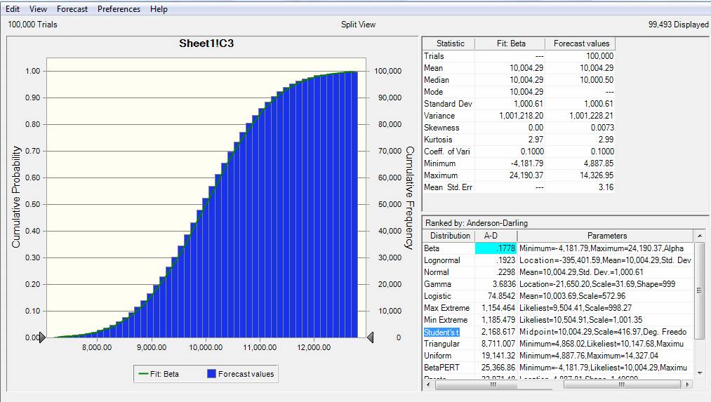
It is interesting, that when using a commercial package such as Oracle Crystal Ball, if an assumption is defined as a Normal Distribution with a Mean of 10,000 and Standard Deviation 0f 1,000, and a Forecast is created from this input, the best fit for the Forecast is not a Normal Distribution, but a Beta Distribution with alpha = 100 and beta = 100
3. It should be noted however, that a continuous statistical distribution, covers all values of Xi between particular limits, whereas a data set comprises of N (the number of data elements in the set) discrete values. While the theoretical continuous statistical distribution defines a dataset in a very precise way, the generated dataset, with N < infinity, cannot contain every possible value, but this would also have been a characteristic of any dataset created by physical measurement.
4. Monte-Carlo simulation usually selects a random cumulative probability value and then uses this to determine a value Xi. If the Random-Number-Generator is biased in some way, then the distribution of the dataset produced will also reflect this distribution.
5. The papers in this series have used datasets which are based on an equal-probability model. In this model, the theoretical distribution is divided up into N strips of equal probability, and the value of Xi is read at the centre of the strip, with values being read according to the following probability sequence:
1/2N, 1/N + 1/2N, 2/N + 1/2N, 3/N + 1/2N, .. (N-1)/N + 1/2N
Hence, if the number of data values N = 100 then the reference probability sequence would be:
|
0.005 |
|
0.015 |
|
0.025 |
|
0.035 |
|
" |
|
" |
|
" |
|
" |
|
0.995 |
6. A criticism of this approach might be that, if we assume N = 100, then we would expect the lowest value to be selected at Pi = 1/100 = 0.01, whereas the method above makes the selection at Pi = 0.005. However, if this were to be adopted, then the final value (the hundredth value) would be read at a probability of 1.0 which would result in a value of Xi which was impossible to determine, particularly if the original distribution was normally distributed.
< p class = MsoNormal style = "TEXT-ALIGN: justify; mso-margin-top-alt: auto; mso-margin-bottom-alt: auto" >7. It should also be noted that the value of N determines how low, and how high readings are taken. For a Normal Distribution, a value of N = 10,000 would result in values being read with probabilities of 0.00005 and 0.99995, given that the +/- 3 SD points occur at probabilities of 0.00135 and 0.99865, it can be seen that when using a value of N = 10,000 one would be working beyond the three standard deviation points.
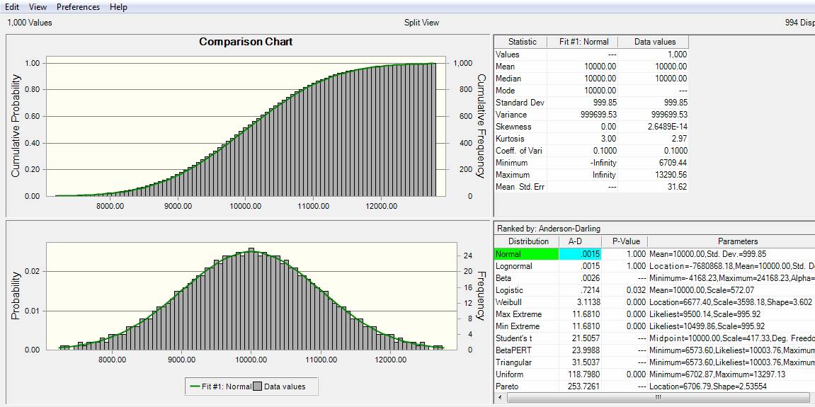
8. If a full data set is created in the manner above, based on the distribution tested above, and the results are then tested in a commercial simulation package it is found that the best-fit resultant distribution is a Normal Distribution with mean 10,000 and Standard Deviation of 1,000.
9. The number of data points N also affects the calculations for Kurtosis and Skew. Kurtosis, based on the fourth moment of the distribution provides a measure of the peakiness or flatness of the distribution. Positive values of Kurt indicate a peaky distribution, while negative values indicate a flat distribution. Skew is based on the third moment of the distribution; with positive skew indicating that the distribution is skewed towards more positive values while negative skew indicates that the distribution is skewed towards more negative values. In both cases the measurement of these third and fourth moment parameters is affect by the value of N. The graph below shows the influence of N upon the value of Kurt.
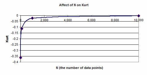
10. In order to counter the influence of N on the values of Skew and Kurt, a standard curve assuming N = 10,000 was employed in producing the results for this series of papers.
(Back)